On this page
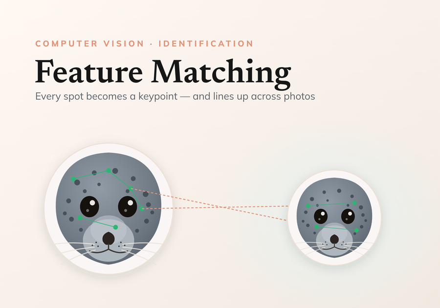
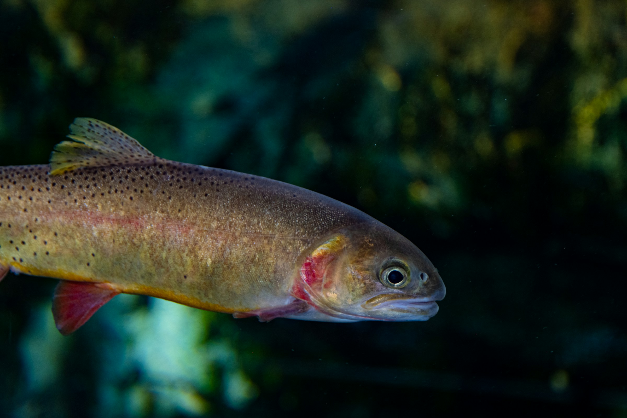
In this post, we will explore a powerful technique widely used for identifying individuals across various species. This method leverages unique physical markings that remain relatively stable throughout an organism’s lifetime, making it effective for species with distinct patterns. For instance, whale sharks, trout, turtles, and seals all possess unique spot or scale patterns that lend themselves well to this computer vision approach.

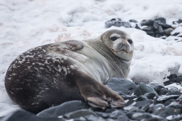
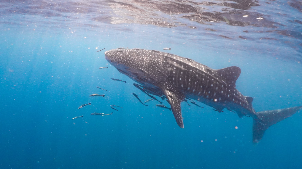
By harnessing these identifiable features, researchers and conservationists can track and monitor individual animals, contributing to our understanding of biodiversity and aiding in conservation efforts. Join us as we delve into the intricacies of this technique and its applications in wildlife identification.
Local Feature Matching
Image matching in computer vision is a fundamental task that involves comparing and identifying similar regions or objects within images. This process is crucial for various applications, including object recognition, image stitching, 3D reconstruction, and more. One of the prominent approaches to image matching is local feature matching, which focuses on identifying and matching distinctive features in images.
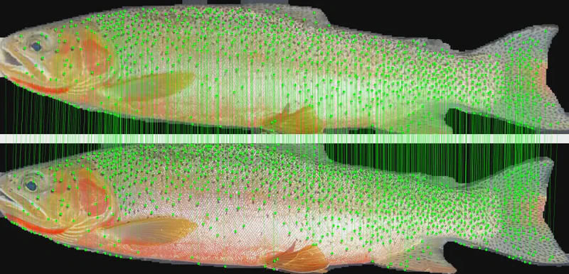
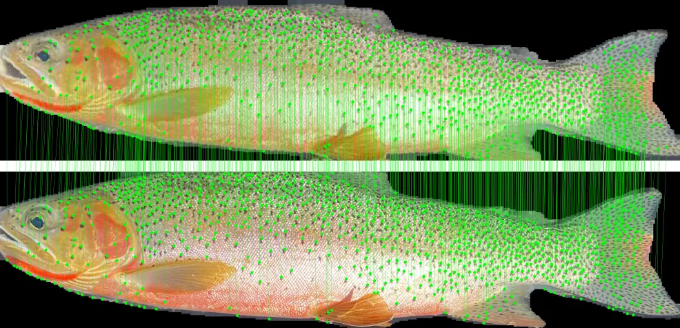
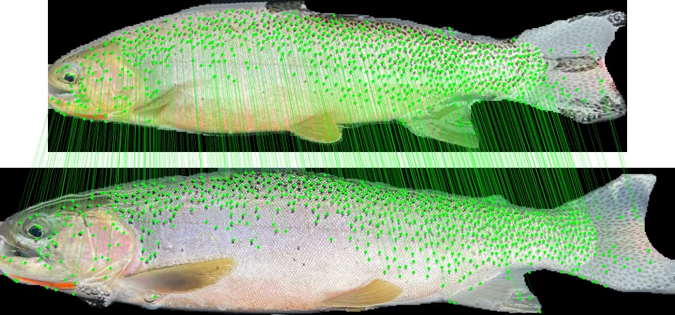
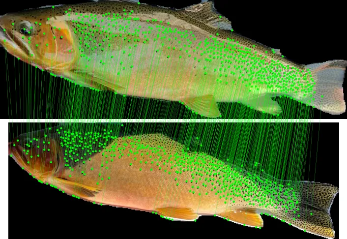
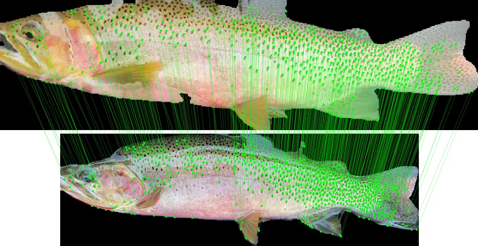
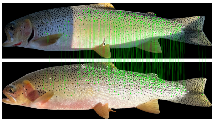 Local feature matching on trout spot patterns
End to end, identifying an individual comes down to four steps:
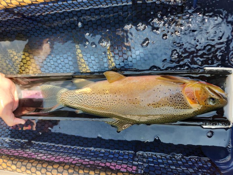
 From a field photo to an identification, at a glance
Here is that same pipeline on a real cutthroat trout — from a raw field photo to a confirmed match against another sighting of the same fish:
Overview of Local Feature Matching
Local feature matching involves several key steps:
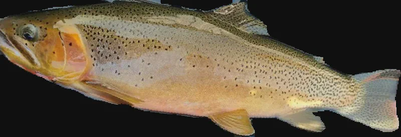
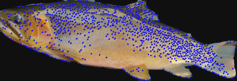
 The local feature matching pipeline, stage by stage
1 · Feature Detection — find keypoints in each image: specific points likely to be stable and distinctive. Common classical detectors include:
- Harris Corner Detector: Identifies corners in the image.
- SIFT (Scale-Invariant Feature Transform): Detects keypoints invariant to scale and rotation, focusing on areas of high contrast — the gold standard for classical local feature extraction.
- DISK (Dense Image Keypoint): Generates dense keypoints across the image, capturing a wide range of features.
- ALIKED (A Local Image Keypoint Descriptor): Emphasizes local image characteristics for robust matching.
State-of-the-art methods now lean on deep-learning features, but classical methods remain strong contenders for feature extraction.
2 · Feature Description — describe the patch around each keypoint as a vector that captures its appearance. Common descriptors include:
- SIFT Descriptors: A vector representation of the local image patch.
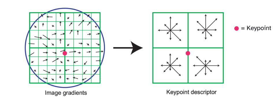 SIFT descriptors describe the direction and magnitude of gradients
- DISK Descriptors: Work in conjunction with the DISK keypoints for a rich representation of local features.
- SuperPoint: A deep-learning approach that produces both keypoints and descriptors in a single network, robust to many transformations.
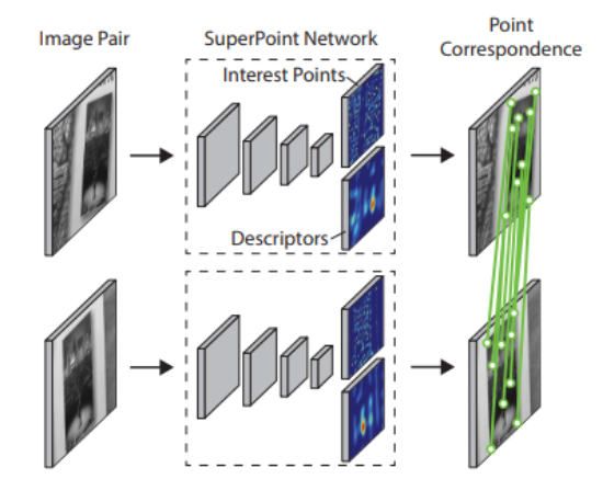 Superpoint Deep Learning Model Architecture - Computes keypoints and descriptors in a single forward pass
3 · Feature Matching — with keypoints and descriptors from both images, pair them up. Tap each approach to compare:
Computes the distance between every pair of descriptors and keeps the closest. Exact and simple, but the cost grows quickly with the number of keypoints.
A neural network that matches features using both local descriptors and global context, making it robust to occlusions and changing viewpoints — state of the art, but heavy.
A lightweight, adaptive successor to SuperGlue: it keeps the accuracy while running fast enough for real-time use, even on modest hardware.
4 · Filtering Matches — not every match is reliable, so filters weed out the weak ones:
Lowe's test, from SIFT: compare the closest match's distance to the second-closest. If the ratio is small enough, the match is distinctive enough to trust.
Random Sample Consensus — fits a geometric transformation to the matches and discards the outliers that don't agree with it.
5 · Geometric Verification — finally, check that the surviving matches are consistent with a single geometric transformation (a homography or affine warp). This eliminates false matches that look similar but don’t fit the overall geometry, refining the result.
Applications of Local Feature Matching
Local feature matching is widely used in various applications, including:
Image stitching
Combining multiple overlapping images into a single panoramic view.
Object recognition
Identifying and classifying objects within images by their distinctive features.
3D reconstruction
Building 3D models from multiple 2D images of the same scene.
LightGlue
LightGlue is a modern feature matching model designed to provide efficient and accurate matching of keypoints in images. It is an evolution of the SuperGlue model, which leverages deep learning techniques to enhance the quality of feature matching by considering both local features and global context. LightGlue is specifically optimized for real-time applications, making it suitable for scenarios where computational resources are limited or where speed is critical, such as in mobile devices or embedded systems.
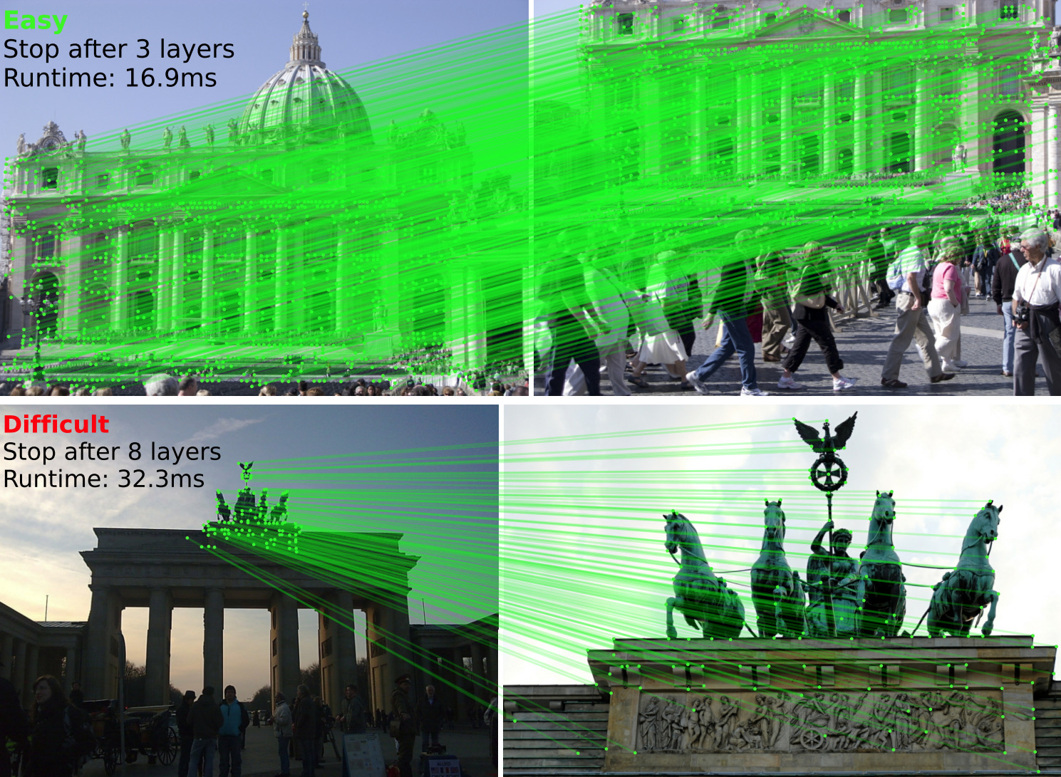 LightGlue example from their GitHub repository
The model operates by first extracting keypoints and their descriptors from input images, similar to traditional feature matching methods. However, it then employs a lightweight neural network architecture to refine these matches, ensuring robustness against occlusions, varying viewpoints, and other challenges commonly encountered in image matching tasks. By balancing accuracy and efficiency, LightGlue enables high-quality feature matching while maintaining fast processing times, making it a valuable tool in various computer vision applications, including augmented reality, robotics, and image stitching.
Metrics
Different metrics can be used to analyze the matching scores outputted by the LightGlue matcher. A simple approach is to examine the length of the LightGlue matches, which is an array of match scores that exceed a specific threshold. However, this method does not fully utilize the complete score distribution.
Two more sophisticated metrics are often employed:
- Area Under Curve (AUC): The AUC provides a comprehensive assessment of the matcher’s performance by measuring the area under the Receiver Operating Characteristic (ROC) curve. This metric considers the trade-off between the true positive rate and the false positive rate across all possible thresholds.
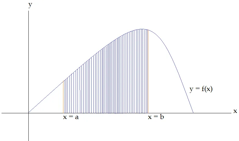 Area Under Curve (AUC) between a and b
- Wasserstein Distance: Also known as the Earth Mover’s Distance, the Wasserstein Distance quantifies the difference between the distributions of match scores for true matches and non-matches (null distribution). This metric captures more nuanced information about the score distributions compared to simply looking at match lengths.
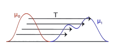 Wasserstein Distance: Required energy to turn the red distribution into the blue distribution
Using these more advanced metrics, one can gain deeper insights into the overall effectiveness and discriminative power of the LightGlue matcher, beyond a basic analysis of match lengths.
We found that the AUC (Area Under Curve) and Wasserstein Distance metrics have very similar discriminative power when applied to the LightGlue matching score distributions. This suggests that either metric can be used to effectively evaluate the performance of the LightGlue matcher, without a significant difference in the insights they provide.
Comprehensive Benchmark
To identify the optimal combination of parameters and feature extractors for your dataset, it is advisable to conduct a comprehensive benchmark that evaluates all potential combinations. This systematic approach will help you determine the most effective configuration.
In our trout identification project, we performed an extensive comparison of the performance of various feature extractors, including SIFT, DISK, ALIKED, and SuperPoint. We tested these extractors on a dataset comprising 250 matching pairs and 250 non-matching pairs. Additionally, we visualized the distributions of matching and non-matching pairs to assess their separation. Our objective is to identify an extractor that yields distributions that are as mutually exclusive as possible, thereby enhancing the accuracy and reliability of individual identification. This thorough analysis will guide us in selecting the best extractor for our specific application.
| Extractor | Precision | Recall | F1 |
|---|---|---|---|
| SIFT | 0.89 | 0.97 | 0.93 |
| DISK | 0.91 | 0.99 | 0.95 |
| ALIKED | 0.91 | 0.99 | 0.95 |
| SuperPoint | 0.91 | 0.99 | 0.95 |
Precision, recall, and F1 for each extractor at 512 keypoints (AUC metric), measured on 250 matching and 250 non-matching trout pairs.
SIFT trails the other three extractors, and the gap widens as you reduce the keypoint budget. The deep-learning extractors (DISK, ALIKED, SuperPoint) hold up well at just 512 keypoints — no better at 1024 — so the smaller budget is the better choice: it streamlines extraction and speeds up every pairwise comparison without costing accuracy.
The next step involves selecting a threshold to identify a new individual. This threshold represents a critical point in the metric score on the distribution graphs, where we aim to optimize the separation between the two distributions. By carefully determining this threshold, we can effectively distinguish between known individuals and new entries, enhancing the accuracy of our identification process. This optimization ensures that we minimize false positives and negatives, leading to more reliable outcomes in our analysis.
Inference Speed
When identifying an individual using Local Feature Matching, the algorithm must compare the input image against all images of known individuals. To be effective, this process needs to be executed rapidly, especially since the known corpus can be quite large.
This approach contrasts sharply with Metric Learning, which scales more efficiently with the size of the known corpus but necessitates a significantly larger dataset of recaptures for model training.
LightGlue, a local feature matching algorithm, is often referred to as “Local Feature Matching at Light Speed” when executed on a GPU.
To better understand the time required for individual identification, we conducted benchmarks to evaluate how the size of the known corpus affects identification speed.
We utilized pre-computed keypoints and descriptors from the trout dataset, which contains approximately 2,750 entries. The identification process involved the following steps:
- Extracting keypoints and descriptors from the input image.
- Performing pairwise matching of the keypoints and descriptors against the entire known corpus (2,750 individuals). The data is batched to optimize the performance of the LightGlue Matcher model on the GPU.
The table below summarizes the results of our benchmark.
| Hardware | Extractor | Keypoints | Batch | Identification | ms / pair |
|---|---|---|---|---|---|
| CPU | ALIKED | 1024 | 1 | 1h 5min | 1418 |
| 1×GPU (T4) | ALIKED | 1024 | 1 | 1min 22s | 29.8 |
| 1×GPU (T4) | ALIKED | 1024 | 64 | 1min 3s | 22.9 |
| 4×GPU (T4) | ALIKED | 1024 | 64 | 20s | 7.3 |
| 1×GPU (T4) | SIFT | 1024 | 64 | 53s | 19.3 |
| 1×GPU (T4) | SIFT | 128 | 64 | 28s | 10.2 |
The pattern is clear: a GPU is the single biggest win — roughly 50× faster than a CPU — and from there, a larger batch size, fewer keypoints, or more GPUs each shave off more time. The matchers themselves run at roughly the same speed; at batch size 64 a single pair takes 20–30 ms, which sets the budget for identifying against the whole corpus.
| Dataset size | Comparisons time (ms) |
|---|---|
| 1 | 20ms |
| 10 | 200ms |
| 100 | 2s |
| 1.000 | 20s |
| 10.000 | 3min20s |
| 100.000 | 33min20s |

Identification time scales linearly with the corpus size — a straight line on these log-log axes. Each 10× more individuals costs 10× more time, which becomes impractical for large datasets.
Running LightGlue on a CPU is generally impractical, as it requires an excessive amount of time to process even a single input image. The optimal setup ultimately depends on the specific use case and the available budget for time and resources.
For occasional identification of individuals in images, a CPU may suffice. However, when dealing with a large volume of images, relying on a CPU becomes unfeasible. In such cases, selecting a GPU configuration from the table above is essential to ensure the pipeline operates within a reasonable timeframe.
Conclusion
Local Feature Matching is a powerful technique for image matching and animal identification, applicable to a wide range of species with unique and stable body markings. The success of this approach depends on selecting the appropriate keypoints, descriptors, and matcher. While effective, Local Feature Matching can be challenging to implement for very large datasets of known individuals, as it requires pairwise matching against the entire corpus. However, conservationists can leverage this non-invasive technology to accurately re-identify individuals, making it a valuable tool for wildlife monitoring and conservation efforts.
You can try the model yourself on real trout spot patterns — the interactive demo runs the full local feature matching pipeline right in your browser.
Try the interactive demo
See the model in action right in your browser — try it on the built-in examples or your own data. No install, no setup.
Open the demo