

On this page
In this post we’ll walk through the technical development of a bear face recognition system, a critical component of the bear identification system built in close collaboration with the BearID Project NGO.
Our research and software tool will provide a replicable technique and general approach that can be applied to other species beyond bears, which could aid conservation efforts worldwide.
– BearID Project
For the full picture, here is the bear identification pipeline. Tap through for the project:
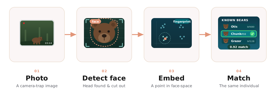 Photo → detect face → embed → match against known bears
Project Scope
While many species boast distinctive fur patterns for identification, brown bears lack consistent and unique markings. Furthermore, their weight can fluctuate significantly between seasons and throughout their lifetimes. Consequently, facial recognition emerges as a valuable alternative for individual identification.
In this article, our attention is directed towards the final phase of the bear identification system, specifically the recognition of bear faces.
The initial stage entails acquiring a mapping capable of embedding bear faces into a high-dimensional space, facilitating the clustering of individuals.
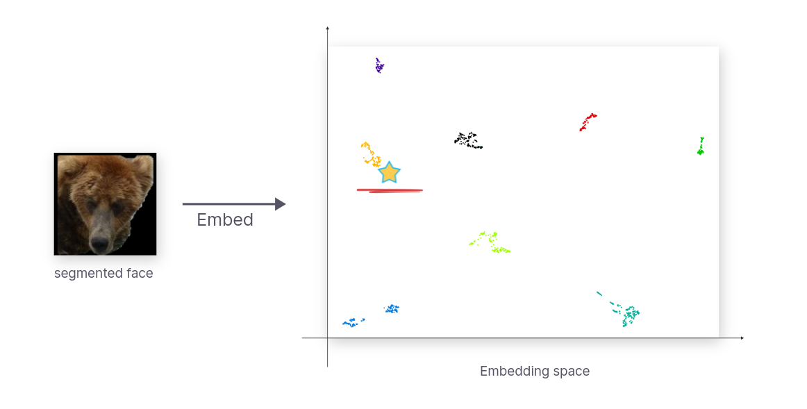 Embedding bear faces into a high dimensional space
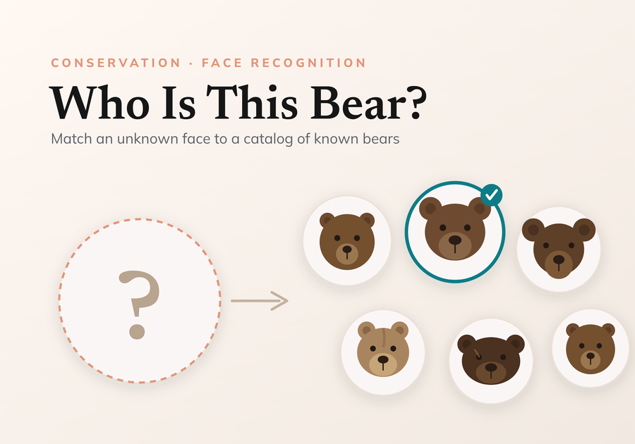
Subsequently, we leverage this learned mapping to execute queries and retrieve the closest matching individuals.
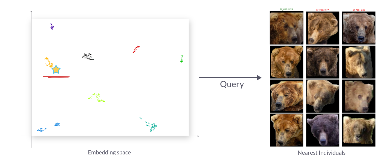 Retrieving closest individuals from the learned mapping
Our collaboration with The BearID Project aims to significantly enhance their current model performance, which currently stands at accuracy@1 (top-1): 0.649 and accuracy@5 (top-5): 0.707.
Provided Dataset
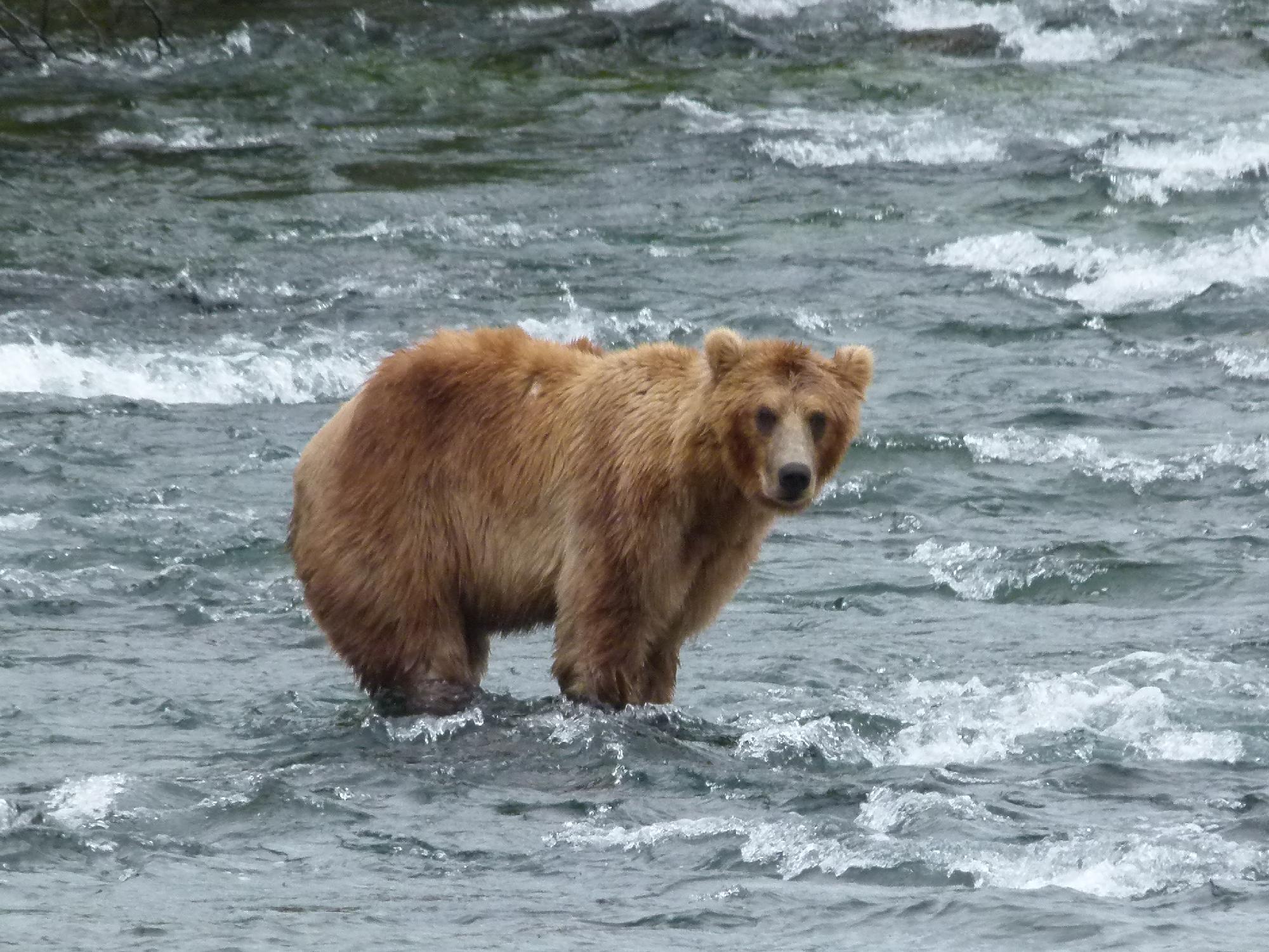
The BearID Project has compiled a collection of bear images, showcasing their facial features, captured over recent years in forests across British Columbia and Brooks Falls.
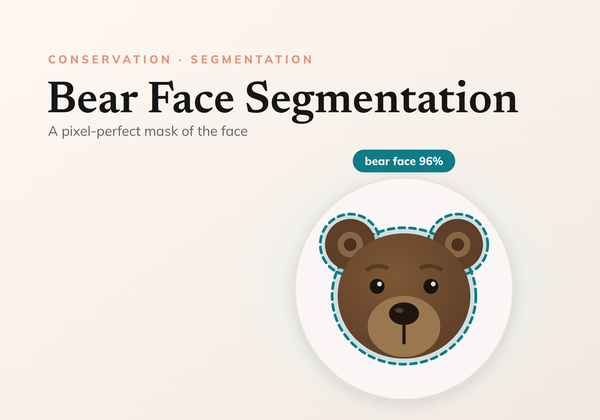
After the development of the bear face segmentation system, as detailed in a prior blog post, we successfully generated approximately 4700 bear face images, representing a total of 132 individuals.
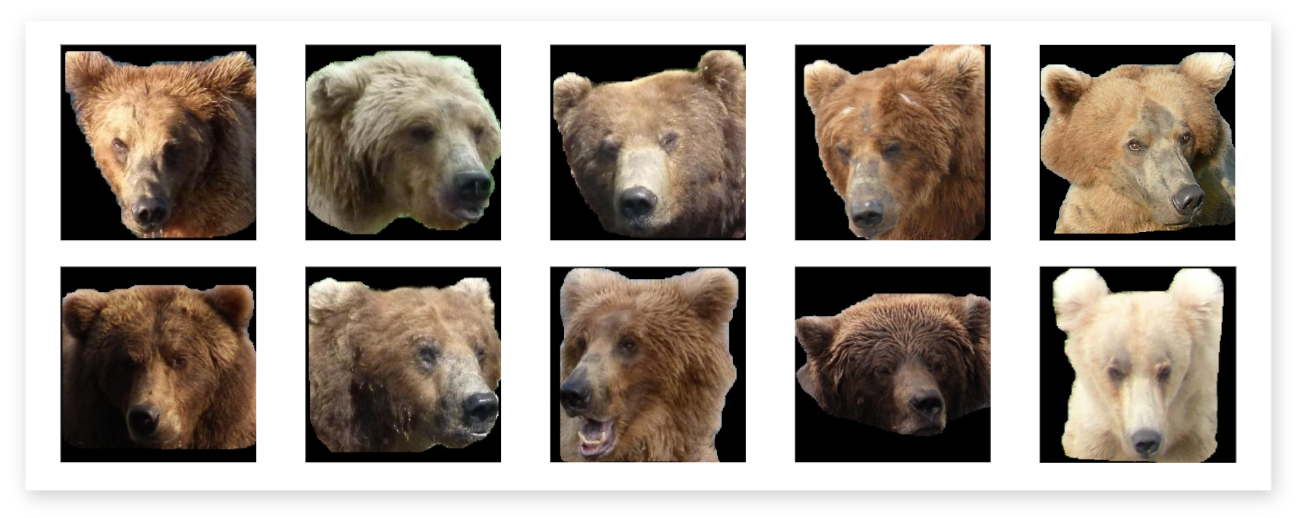 Generated bear faces by the segmentation model
Bursts of images
When encountering a bear, photographs or camera traps often capture multiple images of the same individual in very similar poses. Proper handling of these bursts of images during data splitting is crucial. Neglecting this step may lead to train/test data leakage, which can cause the model to inaccurately overreport its performance.
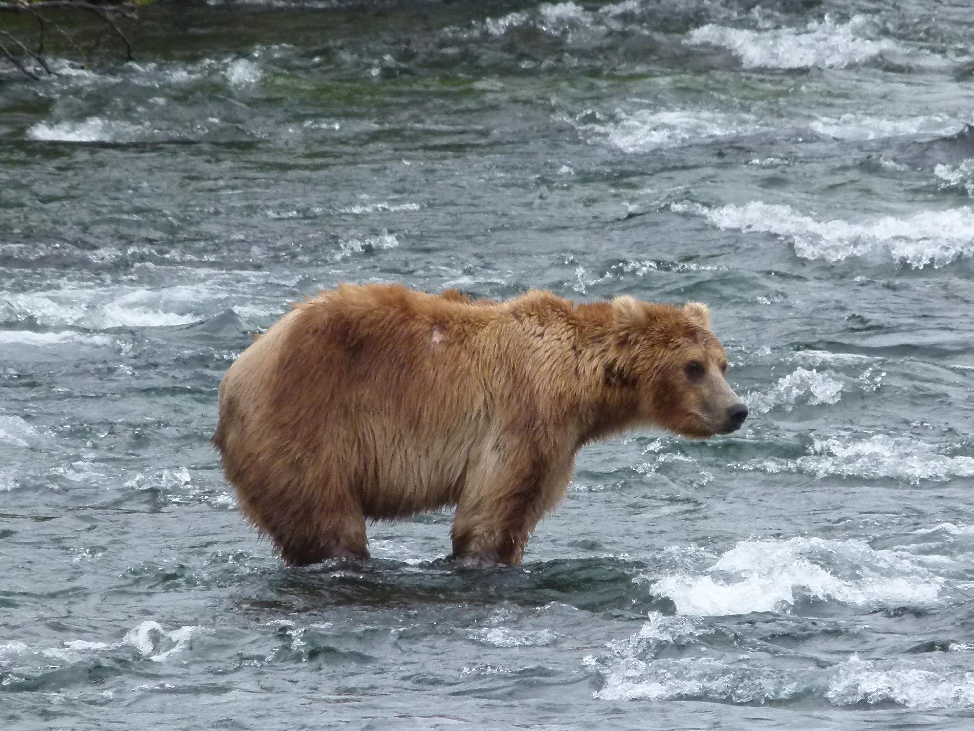
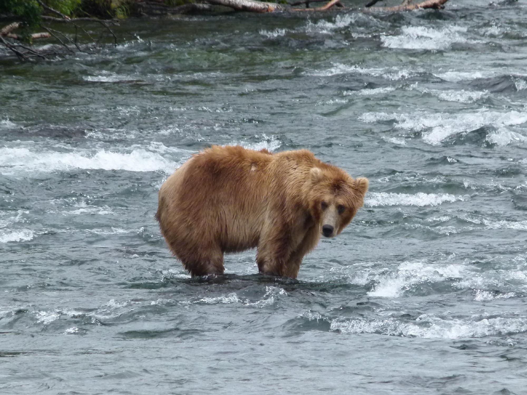
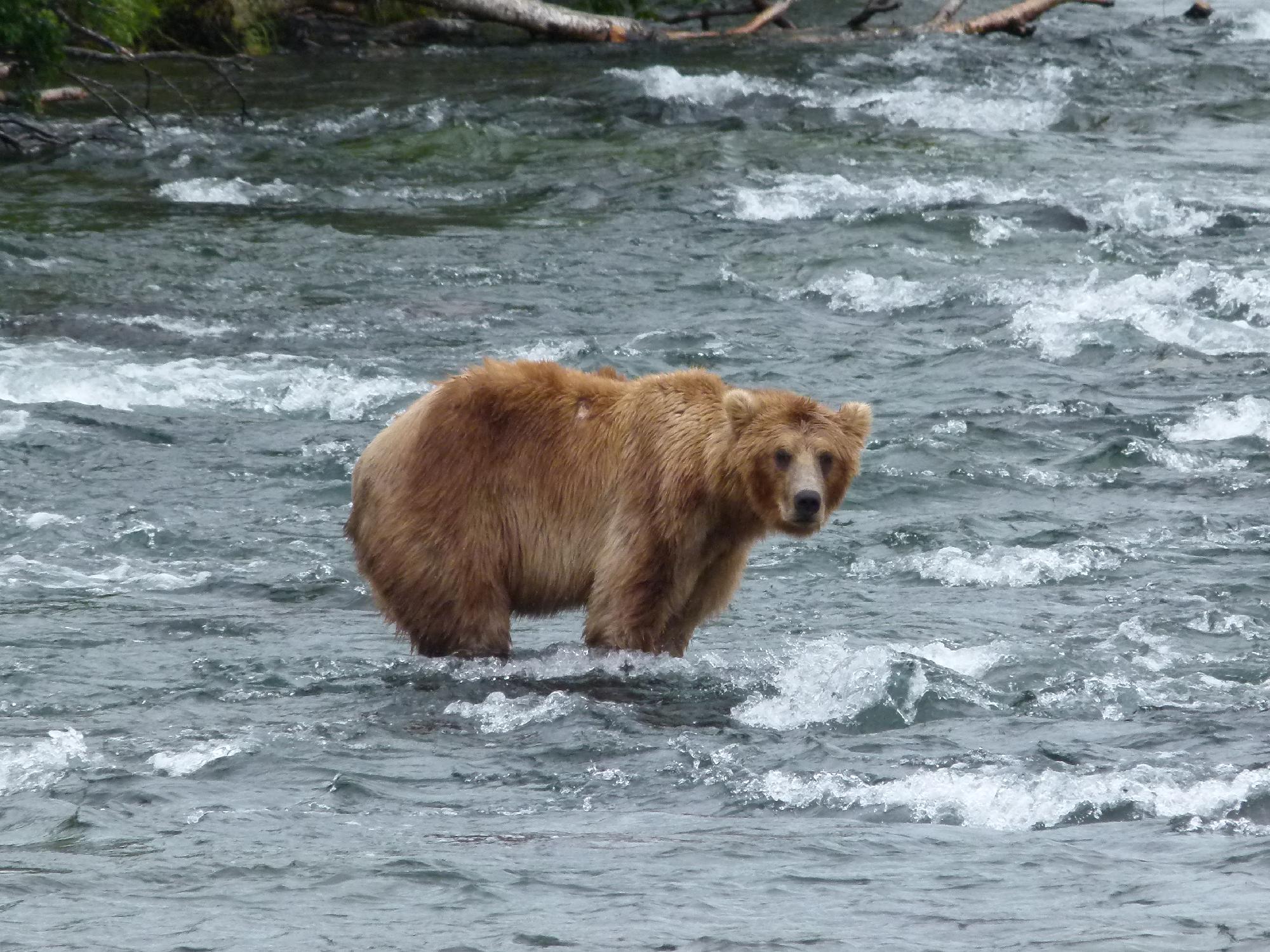
Individual counts distribution
The curated dataset primarily consists of only a few image faces for most bears, posing a potential challenge for accurate identification. Conversely, some bears have hundreds of image faces, largely derived from bursts of images captured during encounters. Below, we present a distribution plot of individual counts to provide further insight into the data.
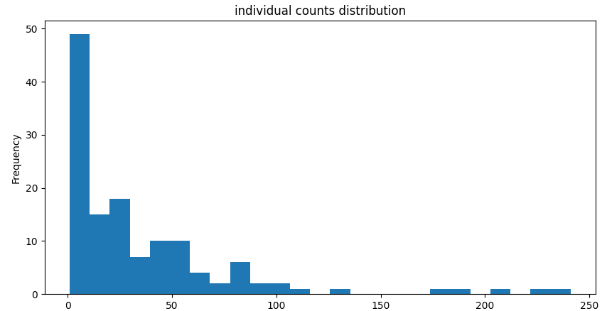 Individual counts distribution - How many image faces per individual?
Re-identification
Re-identification (re-ID) means recognizing and tracking individual animals across camera traps and over time, letting researchers study behaviour, population dynamics, and migration. For brown bears, which lack unique fur markings, the signal lives in the face.
Animal re-ID is harder than the person or object version:
Variable appearance
Fur colour, markings, and physical condition (injuries, season) all change over time.
Field conditions
Camera traps face shifting light, weather, and vegetation that degrade image quality.
Species variability
Different species have different morphologies and behaviours, needing tailored models.
The approach is two familiar steps: a deep network (a CNN) extracts discriminative features from each image, then those features are matched, by nearest-neighbour search or clustering, to link the same individual across images. The payoff for conservation:
Population monitoring
Estimate population sizes, track trends, and gauge the impact of human activity.
Behavioural studies
Follow individuals over time to study movement, habitat use, and social interactions.
Conservation planning
Pinpoint key habitats and corridors to target conservation effort.
Closed, open, and disjoint sets
How identities overlap between training and testing shapes the whole problem:
Closed set
Every identity seen at test time was in the training gallery, so the system only recognizes a fixed, known set.
Open set
Test data may contain new identities, so the system must match the known and flag the unknown.
Disjoint set
Training and test identities don't overlap at all, the hardest, most realistic case for a changing population.
Data Modeling
Data Splits
We opted to create two distinct splits to assess the performance of the identification system in real-world scenarios:
- Open-set split: This split includes a portion of newly introduced identities in the testing phase, simulating encounters with previously unseen entities.
- Disjoint-set split: In this split, the training and testing datasets comprise entirely different identities, mimicking scenarios where the system encounters novel entities during deployment
To avoid data leakage in the open-set split, we implemented a careful splitting strategy based on both camera reference and date. This ensures that bursts of images captured by the same camera at the same time are consistently grouped into the same split (train, validation, or test).
Metric Learning
Overview
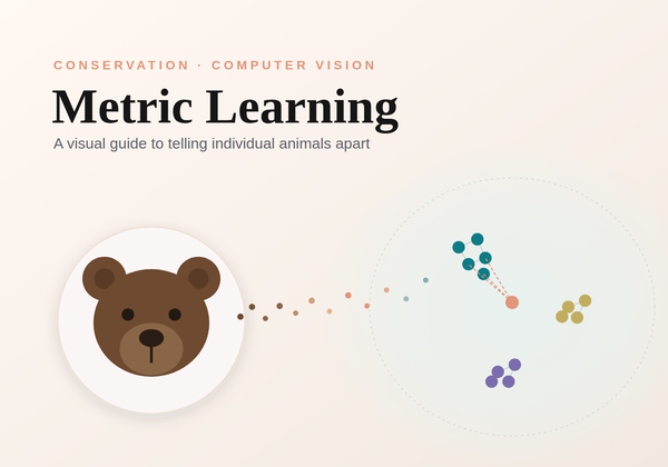
Metric learning is a machine learning paradigm focused on learning a distance metric or similarity function directly from data. Instead of relying on predefined distance measures, metric learning algorithms aim to discover a distance metric that optimally represents the underlying structure or relationships within the data. The goal is to ensure that similar instances are mapped closer together in the learned metric space, while dissimilar instances are pushed farther apart. Metric learning has applications in various domains, including image retrieval, face recognition, clustering, and classification, where accurately capturing the similarity or dissimilarity between data points is crucial for task performance.
Learning a metric space to embed bear faces
Losses
The loss function guides how the embedding space is shaped, pulling similar faces together and pushing different ones apart. We compared four common choices; tap each:
Pulls similar pairs together and pushes dissimilar pairs apart in the embedding space.
Uses (anchor, positive, negative) triplets so the anchor sits closer to the positive than the negative by a set margin, more discriminative than pairs alone.
Gives each class a circular boundary whose radius adapts to its spread; robust to noisy data and large intra-class variation.
Adds an angular margin on a hypersphere, minimizing intra-class and maximizing inter-class angles. Especially strong for faces.
Evaluation Metrics
Main metric - Accuracy@k
Accuracy@k asks a simple question: is the correct individual among the model’s top k ranked matches? It suits retrieval-style tasks where only the top results matter. We track accuracy@1, @3, @5, and @10 throughout both training and evaluation.
Model Topology
The model architecture we adopted consists of a common pretrained backbone, complemented by a compact embedder head, as illustrated below:
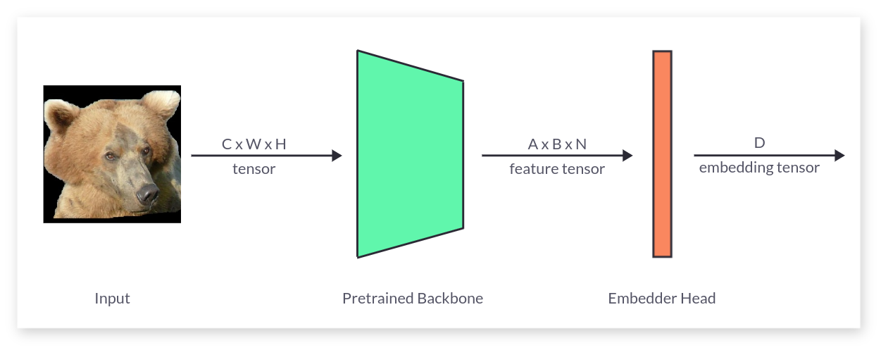 Model Topology - Backbone (trunk) and embedder head
Training
The training process is executed across two GPUs for over 100 epochs. Throughout training, evaluation metrics are continuously monitored, and we save the weights of the best-performing model. Training halts if there’s no improvement in model performance beyond a specified threshold, determined by the patience parameter.
We adopt different learning rates for training the backbone and the heads. This decision stems from the fact that the backbone is typically pretrained on large datasets for feature extraction, whereas the embedder is trained from scratch for the specific task. Typically, we employ a learning rate ratio of 10 to 100 between the backbone and the embedder to effectively balance the learning rates and ensure optimal training dynamics.
Metric Space Visualization - Embeddings
We visualize the metric spaces using UMAP, a versatile manifold learning and dimension reduction algorithm, and save the visualizations after every epoch. This enables us to track and evaluate the improvement of the embedder over time.
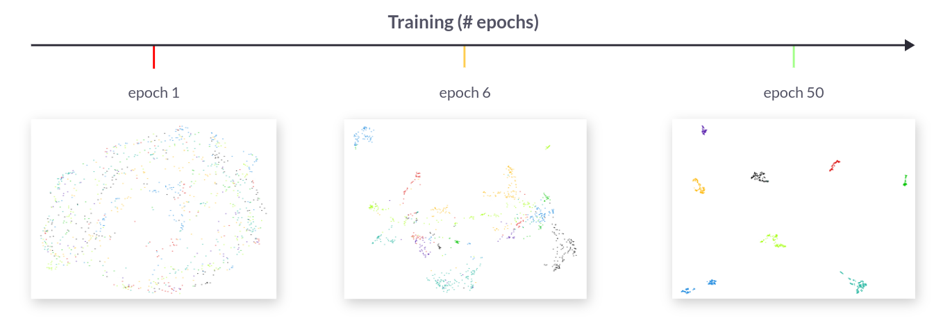 Embeddings over training time
Hard Negative Mining
Hard negative mining focuses training on the most difficult, easily-confused examples, the ones contributing most to the loss. Concentrating on these ambiguous cases yields more discriminative embeddings, uses the training data more efficiently, helps with class imbalance, and improves robustness to noise.
Baseline
A baseline was quickly established using a pretrained ResNet18 as the backbone and a Circle Loss for 1 epoch.
| Split | Backbone | Loss | Epochs | accuracy@1 | accuracy@3 | accuracy@5 | accuracy@10 |
|---|---|---|---|---|---|---|---|
| Disjoint Set | ResNet18 | Circle Loss | 1 | 43.9 | 56.0 | 62.7 | 70.0 |
| Open Set | ResNet18 | Circle Loss | 1 | 54.0 | 66.2 | 71.0 | 79.6 |
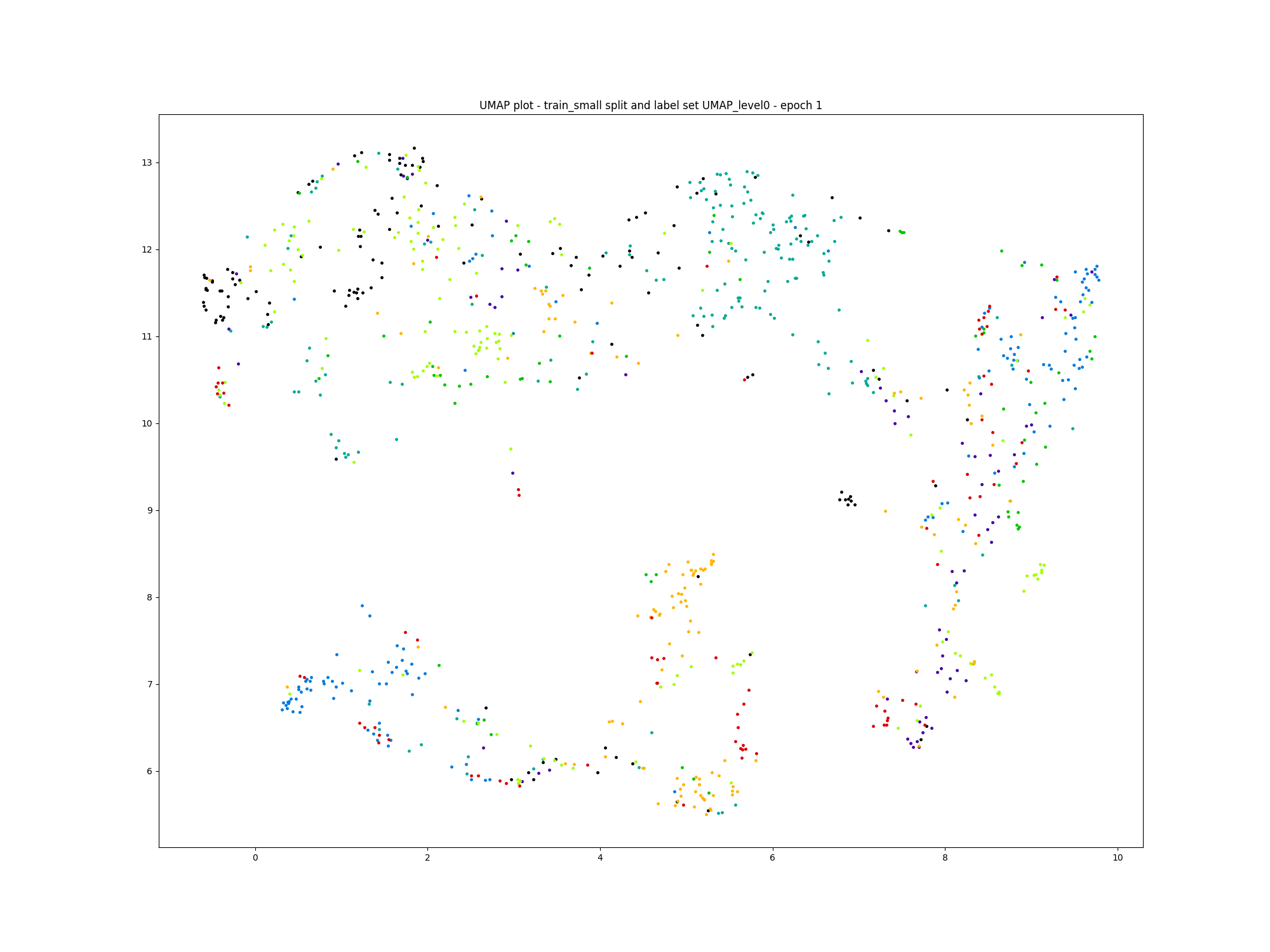 Visualizing the Learned Metric Space: Clusters Yet to Emerge
The approach shows great promise, and selecting the appropriate hyperparameters was key in maximizing the model’s performance
Hyperparameter Search
After configuring experiment tracking, we conducted a random hyperparameter search across the following parameter space:
- backbones: ResNet18, ResNet50, Convnext_tiny, Convnext_large
- losses: tripletmargin, circle, arcface
- learning rates
- weight decay
- mining strategies: easy, semi hard, hard
- embedder’s depth
- optimizers: Adam, SGD, etc
- embedding size; 512, 1024, 2048
- data augmentation steps: rotation, color jitter, etc
We randomly sampled configurations from this parameter space and conducted training sessions for a few days on two GPUs.
Best Model
The winning combination comprises a convnext_large backbone paired with an arcface loss, employing a hard mining strategy, and trained using the Adam optimizer.
| Split | Backbone | Loss | Epochs | accuracy@1 | accuracy@3 | accuracy@5 | accuracy@10 |
|---|---|---|---|---|---|---|---|
| Disjoint Set | Convnext_large | ArcFace Loss | 200 | 95.5 | 96.5 | 97.3 | 98.5 |
| Open Set | Convnext_large | ArcFace Loss | 200 | 95.0 | 95.5 | 95.9 | 96.8 |
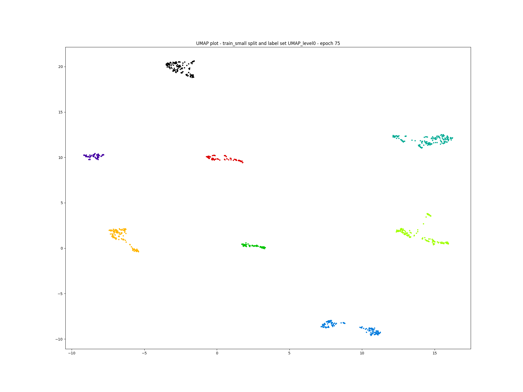 Visualizing the Learned Metric Space: Clusters have emerged
This robust model excels in identifying bears with exceptional accuracy, even in disjoint and open set scenarios, representing a significant advancement over the existing solution developed by BearID. Additionally, we opted to forego the face alignment stage, deeming it unnecessary due to the superior performance of our current approach.
Conclusion
In this guide, we’ve walked through building an open-source model for animal re-identification, applied here to brown bear faces. Deployed with The BearID Project to monitor bear populations in Canada, it is a clear step up from the previous solution, and the same approach can be adapted to other species.
You can try the recognizer yourself on real bear faces; the interactive demo runs right in your browser.
Try the interactive demo
See the model in action right in your browser. Try it on the built-in examples or your own data. No install, no setup.
Open the demo